nano-vllm code walkthrough

vLLM is a beast with 100K+ lines of code, so it’s really challenging to read and learn. Fortunately, there is a great project, nano-vllm (https://github.com/GeeeekExplorer/nano-vllm), which only has a couple thousand of lines, while still keep the skeleton of the real vLLM. In this blog I will firstly explain the key ideas of vLLM, and see how they’re implemented in the nano-vllm project.

High level ideas

Block-based memory management

At LLM inference time, the straightforward implementation is that, we feed user’s prompt to the model, get next token, append the new token to the end of original prompt and feed the new sequence to the model again. Repeat until we get EOS token or reach the max allowed sequence length.

This is not efficient because we keep computing the prefix tokens’ activations again and again. Instead, we can keep the previous computed Keys and Values of the attention layers in a “KVCache”, and every iteration we only need to compute the one new token’s results.

However, the KVCache produces a challenge about GPU memory management. We have to pre-allocate enough memory to avoid fragmentation, but if we always allocate the max allowed sequence length at the beginning of each request, we’re likely wasting a lot of memory unused.

Inspired by the paged virtual memory in operating system, the authors of vLLM invented PagedAttention, which basically means partitioning the kvcache into smaller, fixed-size chunks (pages). We allocate new chunks on demand as the sequences growing, so as a result each sequence may be corresponding to a list of (non-continuous) chunks.

Prefill and decode

This is not the invention of vLLM but it’s critical to understand all the following discussions. At inference time, a request will go through two stages: prefill and decode.

In the prefill stage, the input is the user’s original prompt, we compute all the tokens in parallel, and get the next token as result. Then in the decode stage, we compute one next token at a time sequentially, until we get EOS token.

These two stages have different characteristics. The prefill stage is compute-intensive, while the decode stage is more memory-bound. In real inference system these two stages are usually disaggregated.

This high level idea is not difficult to understand, but there are lots of details/tricks in terms of implementation. So let’s dive into the code of nano-vllm.

Important Python Classes

Sequence

• Sequence represents a request. It has three possible status: WAITING, RUNNING, FINISHED. At the beginning, it is initialized as the original prompt, and new tokens are appended as processing.
• One of the most important fields is block_table, which is a list of block ids and each block contains a constant size (256) of tokens at most.

Block and BlockManager

• Each block has a unique block id, in the range of [0, num_blocks). Here the num_blocks is computed from the available GPU memory. Each block contains at most 256 token ids. Besides token_ids fields, there are two fields hash and ref_count used for prefix caching, which we will talk below.
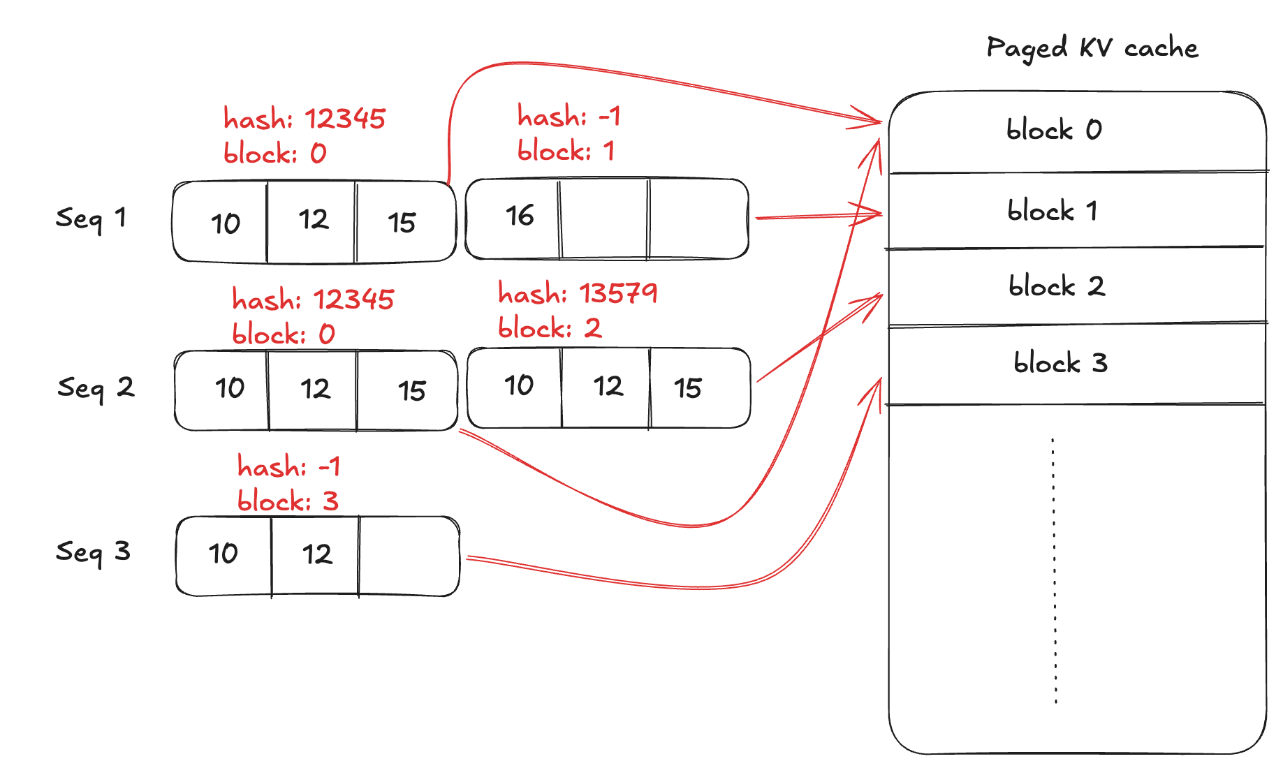
• BlockManager manages the blocks. It maintains free_block_ids and used_block_ids. When we receive a new sequence, we call allocate(self, seq) to allocate proper number of blocks (i.e. ceil(len(seq) / 256) ). And when we finished a sequence the corresponding blocks will be returned to free_block_ids .
• When we allocate blocks for a sequence, we get a list of full blocks (i.e. block contains 256 tokens) and one possible non-full block at the end. For each full block, we compute hash of it’s token ids together with its previous block’s hash. So that each such hash value uniquely defined a sequence prefix. The BlockManager maintains hash_to_block_id , so that if multiple input sequences share same prefix, the block_id can be reused.
• Also, during the decoding, the sequence is growing. Once the tail block becomes full, we also compute its hash and update the hash_to_block_id , then allocate a new tail block.

See below diagram as an example. We have three sequences [10, 12, 15, 16], [10, 12, 15, 10, 12, 15], [10, 12]. The block size is 3. The block_table of these 3 sequences are [0, 1], [0, 2], [3], respectively. Note that the first block of seq1 and first block of seq2 shares same cache page. But the second block of seq2 doesn’t, because its hash is different.

Scheduler

• The scheduler maintains two queues waiting (sequences need pre-filling) and running (sequences need decoding.) When a new request comes, the add(self, sequence) is called, and the request goes to waiting queue.
• Every time when the schedule() is called, it will return either a batch of pre-filling task, or a batch of decoding task (but never mixed). The scheduler will try to collect as many sequences in the waiting queue as possible, and return a batch of prefilling tasks. If no prefilling task at all, it will collect decoding tasks. (I skipped preempt logic here for simplicity)

LLMEngine

• For each new prompt, LLMEngine call tokenizer, then call scheduler.add(seq)
• It repeatedly call scheduler.schedule() to get a batch of prefilling or decoding tasks, then call model_runner.call() to run the model, then call postprocess() to append new tokens to the sequences.

Model Runner in details

For the model runner, I will be focusing on the attention computation, because that’s the part which has most difference for training vs inference (in my opinion).

At training time, the input shape of attention layer is typically [batch, seq_len, num_heads, heads_dim]. Here all the sequences have same length because we can just prepare the training data in that way.

However, at inference time, the sequence length varies. Assuming we collected a batch of sequences for the prefilling, we will see a “rugged” shape of inputs. One straightforward way is padding all sequences to the longest sequence, hence we can still use the classic approach. But a more efficient way is to “squash” the sequences into a single long one, and relying on the mask to dictate which tokens should be attended.

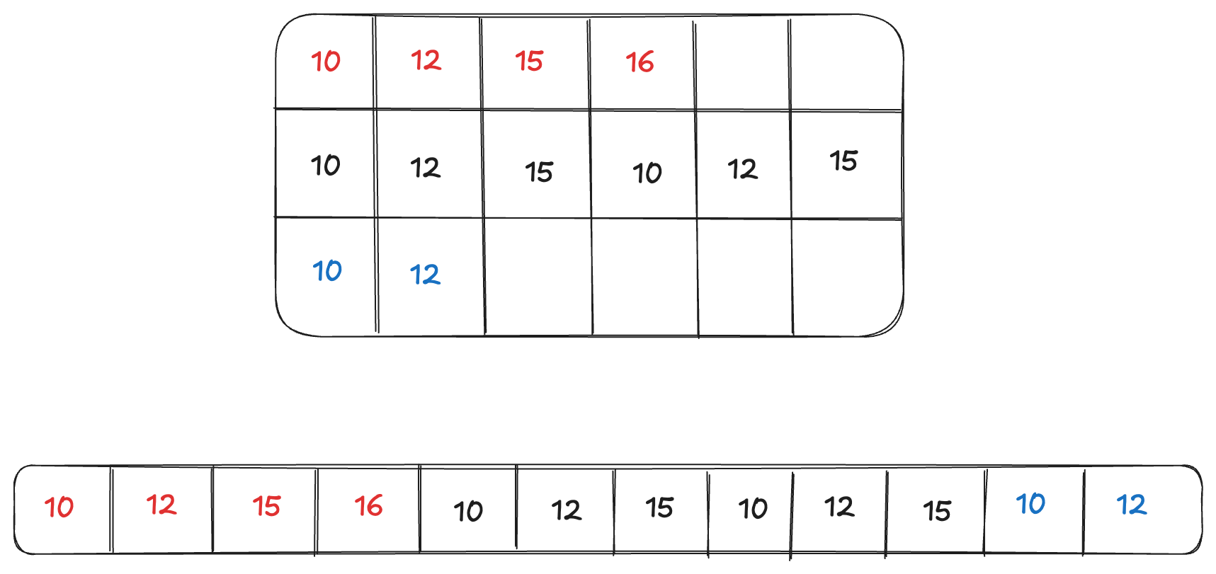
Rugged and Squashed representation

nano-vllm utilize variants of flash attention implementations: flash_attn_varlen_func for prefilling, and flash_attn_with_kvcache for decoding.

Prefill stage

Let’s take a look at the signature of flash_attn_varlen_func :

flash_attn_varlen_func(q, k, v,
		max_seqlen_q, cu_seqlens_q,
    max_seqlen_k, cu_seqlens_k,
    softmax_scale, causal, block_table)

This call is in the forward call of Attention layer in attention.py , but the parameters that are same across all attention layers are prepared in perpare_prefill() in model_runner.py, saved as a global context. These includes max_seqlen_q, cu_seqlens_q, max_seqlen_k, cu_seqlens_k, block_table. These parameters scared me at the beginning, but once it started to make sense, all the puzzled resolved automatically.

There are actually two scenarios that I found maybe easier to discuss separately:

Case 1: No prefix found in cache.

For this case, we need compute all the tokens from scratch. Let’s examine the params one by one:

• q: As mentioned above, we put all sequences into a single one, so q’s shape is [total_tokens, num_heads, heads_dim].
• cu_seq_lens_q: has length (num_sequences + 1). It’s the cumulated lengths of each sequence in q. For example, if we have three sequences with length 2, 5, 3, then the cu_seq_lens_q will be [0, 2, 7, 10]. By doing that we know each token in q belongs to which sequence.
• k and v: contains squeezed k and v, similar as q. For this no-cache-found case, the logical length of k/v is same as q. And we pass-in the actual physical k and v tensor, which is continuous in memory so the performance is better than use paged cache blocks.
• cu_seqlens_k: similar as cu_seq_lens_q . Btw we don’t need another cu_seqlens_v because k and v always have same length.
• max_seqlen_q, max_seqlen_k: the max sequence len in q and k, used by flash attention internal implementation. We skip the details for now.
• softmax_scale: for example, use the sqrt(D) as in original transformer paper.
• causal: set to true for causal language model like here, we don’t see the future tokens.
• block_table: pass in None for this case, indicates we don’t use cache.

Case 2: Some prefix(es) found in cache.

• q: For this case, we exclude the prefix tokens that are found in cache. So the q’s length q.shape[0] is less than total length of sequences.
• cu_seq_lens_q : similar accumulated lengths. Note cu_seqlens_q[-1] is q.shape[0]
• k and v : though q is shorter, logically we should still use the full-length k/v, because the tokens in q need to attend all previous tokens in the sequence. So the “logical” length of k/v should be same as case 1. However, the physical data is scattered in the cache pages, so here we pass in the address of k_cache and v_cache , and use the last block_table parameter to indicate which cache pages belong to this sequence.
  • k_cache and v_cache has shape [num_blocks, block_size(256), num_heads, head_dim] . That means, for example k_cache[i] is the block i of k_cache.
• cu_seqlens_k, cu_seq_lens_q: same as case 1, note cu_seqlen_k[-1] > cu_seqlens_q[-1]
• block_table: 2D tensor has shape [num_seqs, max_blocks_per_seq]. Its values are the block ids. (use -1 for padding) Conceptually we can use it to locate the blocks in k_cache/v_cache, and “stitch” the blocks to get the full k/v sequence. (It’s not literally implemented that way in flash attention code, of course)

For both cases, the output shape is same as q.

Decode Stage

Now the decoder part is much clearer, we use another flash attention variant:

flash_attn_with_kvcache(q, k_cache, v_cache,
	cache_seqlens, block_table, softmax_scale, causal)

For this case,

• q has shape [num_seqs, 1, num_heads, head_dim] . Note that the q.shape[1] is 1, because there is always one new token for each decoding iteration.
• k_cache, v_cache , block_table is same as the above Prefilling case 2.
• cache_seqlens is a 1D tensor of length num_seqs, and cache_seqlens[i] means the current number of tokens for sequence i. This is needed because the cache block may be only partially filled.

Tensor Parallelism

nano-vllm also support tensor parallelism, i.e., the tensors are partitioned to multiple GPUs. Let’s examine how this was achieved for each layer.

Embedding Layer (VocabParallelEmbedding)

For the embedding layer, the embedding matrix are partitioned by the token ids axis, i.e. each GPU loaded a range of token ids’ embeddings. For the forward call, it masks the input token ids outside of its own range, only to apply the embeddings belongs to its range. Then use dist.all_reduce() to collect the results.

MLP Layer (Qwen3MLP)

The key parts are two linear layers, up and down. The up matrix shape is [hidden_size, intermediate_size], and the down matrix is [intermediate_size, hidden_size]. The input will be multiply the first matrix, then apply a non-linear transformation, then multiply the second matrix. (I’m a bit simplified here but the idea is same.) Now the problem is how to partition these two matrixes.

Turns out we should partition the up matrix by column (ColumnParallelLinear) and the down matrix by row ( RowParallelLinear ), so that each GPU will hold up matrix [hidden_size, intermediate_size / world_size] and down matrix [intermediate_size / world_size, hidden_size] .

Let’s say the input shape is [tokens, hidden_size] . For the first matmul we don’t need do anything special, then each GPU got a result of size [tokens, intermediate_size / world_size]. Then we do the second matmul, each GPU got a result of size [tokens, hidden_size]. However each GPU has only partially data now, we need sum them together by using dist.all_reduce(). Now all the GPUs have the same correct result.

Attention Layer (Qwen3Attention)

We partitioned the qkv projection matrix by the num_head axis (essentially the ColumnParallelLinear ), so each GPU handles a subset of heads. Obviously the attention computation of each head is independent. The only reduce happens when we do the last O projection. Similar as the MLP layer, we partition the O projection matrix by row, then do a final all_reduce() at the end.

I’m afraid my description about TP may be too simple here. If you don’t quite understand what I’m talking about, there are a lot of great articles about tensor parallelism in LLM on the Internet.

Misc implementation details

Where does k_cache, v_cache in Attention get initialized?

It confused me quite some time, because they’re not initialize in attention.py. The init actually happens in allocate_kv_cache() in model_runner.py , called during ModelRunner.init()

Firstly one big tensor is allocated for the entire KV cache, shaped [2, num_layers, num_blocks, block_size, num_heads, head_dim] - the 2 is for K and V, and the block_size is computed based on available total GPU mem. Then there is a for-loop going through all modules of the model. If one module has k_cache/v_cache attributes, it will be assigned a slice of the big tensor. (I personally don’t quite like this kind of hard-coded name, but it’s simple and working.)

What is the CUDA graph in decode stage, and why not for prefill?

CUDA graph allows us to define a series of kernels (whose dependencies forms a graph) once, then launch the graph multiple times afterward. It can reduce the kernels launch overhead - instead launch multiple kernels from time to time, we just need launch the whole graph once. The limitation is that the input tensor size and address must be static.

In the decode stage, the only different size across different runnings is the number of sequences in a batch, all other shape dimensions are static. So nano-vllm pre-captures multiple graphs for different num_seqs values like [1, 2, 4, 8, 16, .. 512] . At inference time the engine picks the smaller viable one to run.

On the other hand, the sizes of prefill stage is much more variable - different num_seqs, different prompt lengths, etc. So it’s not quite possible to predefine some sizes.

Also, the prefill stage tends to be compute-bound, which means the kernel launch overhead is small comparing with the kernel running time itself. But for the decode stage the kernel launch overhead is significant. (The prefill stage is pretty much matrix-matrix multiplication, while the decoding stage is vector-matrix multiplication.)